8.2.2.2 Detailed Design Procedure

As illustrated in Figure 20, this design example consists of a mechanical component that moves back and forth, an embedded magnet with the south pole facing the printed-circuit board, and a DRV5057-Q1. The DRV5057-Q1 outputs a PWM that describes the precise position of the component. The component must not contain ferromagnetic materials such as iron, nickel, and cobalt because these materials change the magnetic flux density at the sensor.

When designing a linear magnetic sensing system, always consider these three variables: the magnet, sensing distance, and the range of the sensor. Select the DRV5057-Q1 with the highest sensitivity possible based on the system distance requirements without railing the sensor PWM output. To determine the magnetic flux density the sensor receives at the various positions of the magnet, use a magnetic field calculator or simulation software, referring to magnet specifications, and testing.

Magnets are made from various ferromagnetic materials that have tradeoffs in cost, drift with temperature, absolute maximum temperature ratings, remanence or residual induction (B_r), and coercivity (H_c). The B_r and the dimensions of a magnet determine the magnetic flux density (B) produced in 3-dimensional space. For simple magnet shapes, such as rectangular blocks and cylinders, there are simple equations that solve B at a given distance centered with the magnet. Figure 21 shows diagrams for Equation 4 and Equation 5.

Figure 21. Rectangular Block and Cylinder Magnets

Use Equation 4 for the rectangular block shown in Figure 21:

Equation 4.

Use Equation 5 for the cylinder illustrated in Figure 21:

Equation 5.

where

• W is width
• L is length
• T is thickness (the direction of magnetization)
• D is distance
• C is diameter

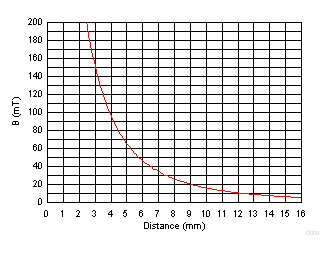
This example uses a cylinder magnet; therefore, Equation 5 can be used to create a lookup table for the distances from a specific magnet based on a magnetic field strength. Figure 22 shows a magnetic field from 0 mm to 16 mm with the magnet defined in Table 2 as C = 4.7625 mm, T = 12.7 mm, and B_r = 1480 mT.

Figure 22. Magnetic Field vs Distance

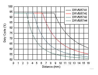
In this setup, each gain version of the sensor produces the corresponding duty cycle shown in Figure 23 for 0 mm to 16 mm.

Figure 23. %D vs South Pole Distance (All Gains)

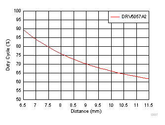
With a desired 5-mm movement swing, select the DRV5057-Q1 with the largest possible sensitivity that fits the system requirements for the magnet distance to the sensor. Assume that for this example, because of mechanical restrictions, the magnet at the nearest point to the sensor must be selected to be within 5 mm to 8 mm. The largest sensitivity option (A1) does not work in this situation because the device output is railed at the farthest allowed distance of 8 mm. The A2 version is not railed at this point, and is therefore the sensor selected for this example. Choose the closest point of the magnet to the sensor to be a distance that allows the magnet to get as close to the sensor as possible without railing but stays within the selectable 5-mm to 8-mm allowed range. Because the A2 version rails at approximately 6 mm, choose a closest distance of 6.5 mm to allow for a little bit of margin. With this choice, Figure 24 shows the %D response at the sensor across the full movement range.

Figure 24. %D vs South Pole Distance (Gain A2)

The magnetic field strength is calculated using Equation 6, where a negative number represents the opposite pole (in this example a south pole is over the sensor, causing the results to be a positive number).

Equation 6.

For example, if the A2 version of the DRV5057-Q1 measured a duty cycle of %D = 74.6% using Equation 1 , then the magnetic field strength present at the sensor is (74.6 – 50) / 1 = 24.6 mT.

Using the lookup table that was used to create the plot in Figure 22, the distance from the magnet at 24.6 mT is D ≈ 8.2 mm.

For more accurate results, the lookup table can be calibrated along the movement path of the magnet. Additionally, instead of using the calibrated lookup table for each measurement, consider using a best-fit polynomial equation from the curve for the desired movement range to calculate D in terms of B.

The curve in Figure 24 is not linear; therefore, the achievable accuracy varies for each position along the movement path. The location with the worst accuracy is where there is the smallest change in output for a given amount of movement, which in this example is where the magnet is farthest from the sensor (at 11.5 mm). Determine if the desired accuracy is met by checking if the needed %D_LSB at this location for the specified accuracy is greater than the noise level (PWM jitter) of 0.1%D. Thus, with a desired accuracy of 0.1 mm, the needed %D_LSB is the change in %D between 11.4 mm and 11.5 mm. Using the lookup table to find B and then solving for %D in Equation 6, at 11.5 mm, B = 11.815 mT (which equates to 61.815%D), and at 11.4 mm B = 12.048 mT (which equates to 62.048%D). The difference in %D between these two points is 62.048 – 61.815 = 0.223%D_LSB. This value is larger than the 0.1%D jitter, so the desired accuracy can be met as long as a %D_LSB is selected that is equal to or less than 0.223 using Equation 2.