SLVA450B February 2011 – April 2021 TL7770-12 , TL7770-5 , TPS3513 , TPS3514 , TPS3606-33 , TPS3613-01 , TPS3617-50 , TPS3618-50 , TPS3619-33-EP , TPS3620-33-EP , TPS3805H33-EP , TPS3808-EP , TPS3818G25 , TPS386000 , TPS386000-Q1 , TPS386040 , TPS386596 , TPS60120 , TPS60121 , TPS60122 , TPS60123 , TPS60124 , TPS60125 , TPS60130 , TPS60131 , TPS60132 , TPS60133 , TPS60140 , TPS60141 , TPS60204 , TPS60205 , TPS60210 , TPS60211 , TPS60212 , TPS60213 , TPS61130 , TPS61131 , TPS62050 , TPS62051 , TPS62052 , TPS62054 , TPS62056 , TPS62110 , TPS62110-EP , TPS62111 , TPS62111-EP , TPS62112 , TPS62112-EP , TPS65000 , TPS65001 , TPS65010 , TPS65011 , TPS65012 , TPS65013 , TPS65014 , TPS65020 , TPS65021 , TPS65022 , TPS65023 , TPS650231 , TPS65023B , TPS650240 , TPS650241 , TPS650241-Q1 , TPS650242 , TPS650243 , TPS650243-Q1 , TPS650244 , TPS650245 , TPS650250 , TPS65050 , TPS65053 , TPS65055 , TPS650830 , TPS65086 , TPS65720 , TPS65721 , TPS65810 , TPS65811 , UC1543 , UC1903 , UC2543 , UCC2946 , UCC3946
3 Example Calculations
Table 3-1 lists the system requirements that necessitate the use of an SVS with 1% accuracy threshold voltage. When the supply voltage falls below 10% of its nominal value of 3.3 V to 2.97 V, the processor should reset. VREF and IS can be found directly from the device data sheet.
| Field | Value |
|---|---|
| IC | TPS3808G01 |
| VREF | 0.405 V |
| IS | ±25 nA |
| VI | 3.3 V |
| VIT | 2.97 V |
| Desired % ACC | 1% |
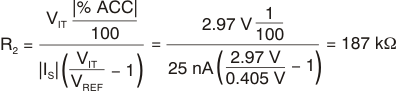
First, calculate R2 to its nearest standard value, using Equation 9.
With R2 known, calculate R1 to the nearest standard value, using Equation 10.

As an effect of using standard-value resistors,
the expected threshold voltage can be found by using
Equation 11.

Then, using Equation 6, the input current is found. IS is evaluated as a positive value to find the maximum amount of current through the divider.
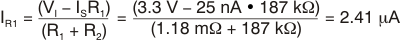
One can also observe that this current is roughly 100 times the leakage, which validates the rule of thumb noted earlier.
Finally, using Equation 5 and Equation 6, Figure 3-1 shows the variation in worst-case accuracy and input current to the divider with R2 ranging from 1 kΩ to 1 MΩ. Note the accuracy is centered on the new calculated VIT: 2.974 V.
 Figure 3-1 Accuracy and
Current Variations through the Divider vs. Resistance of R2
Figure 3-1 Accuracy and
Current Variations through the Divider vs. Resistance of R2Figure 3-1 also clearly illustrates the linear relationship of accuracy and exponential relationship of current to R2 (note the logarithmic axes). This correlation demonstrates the diminishing returns for both an increase and a decrease in the resistance R2. At the lower end, the current increases significantly with a small increase in accuracy. On the high end, the accuracy decreases significantly for small decreases in current. The accuracy from the leakage is nearly always better than what is shown in the graph because the amount of leakage is not always at the worst-case conditions. The current, however, does not vary significantly because the leakage current is virtually always a fraction of the current into the divider.