SLYA051A october 2020 – april 2023 DRV5055 , DRV5055-Q1 , DRV5057 , DRV5057-Q1 , TMAG5170 , TMAG5170-Q1 , TMAG5170D-Q1 , TMAG5173-Q1 , TMAG5273
5 Identifying Sources of Error
To explore the solution further, the DRV5055EVM was modified to use all four sensors with the A1 sensitivity option. A magnet matching the geometry and material in Linear Transit Position Sensing was selected for consistency.
Absolute position of the magnet was driven using a motorized motion controller along a single axis of motion, and the PCB was positioned such that the 8 mm air gap to the magnet was maintained for the full transit.
The captured data helps show the impact of various sources of error which may be present in a design.
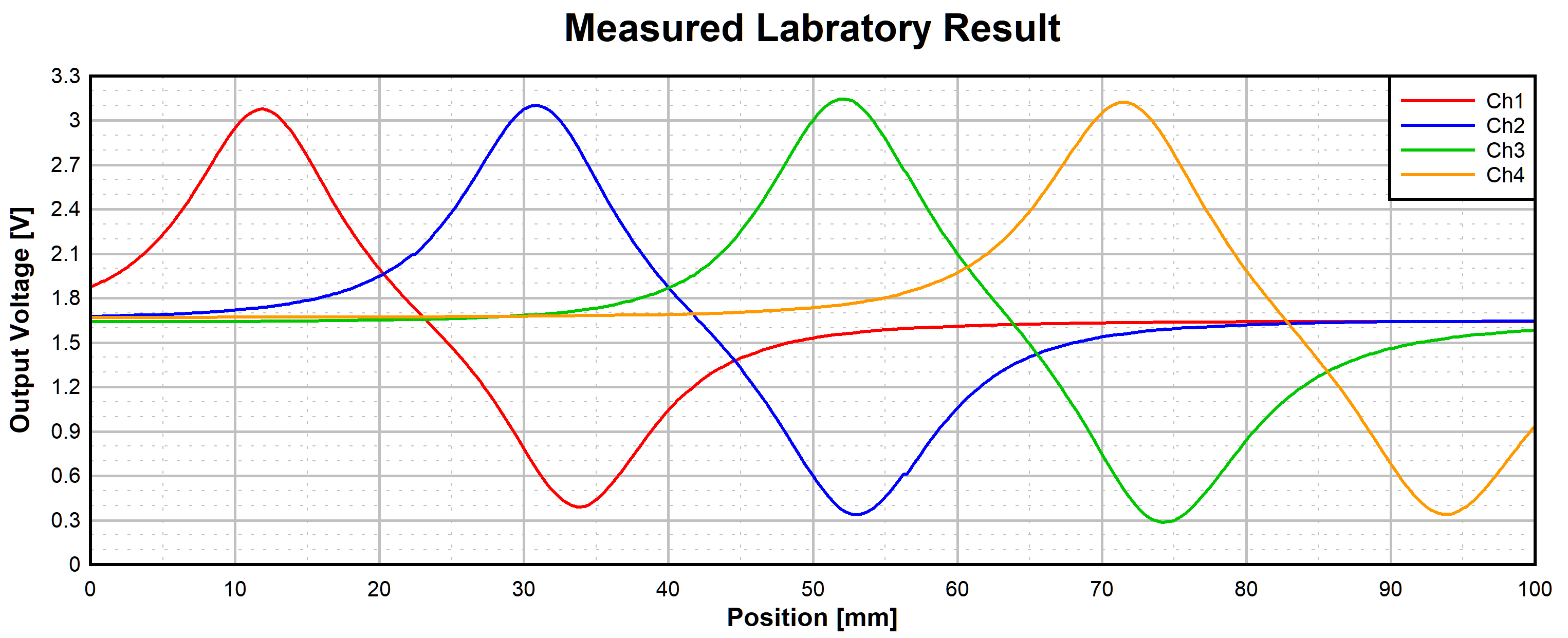
 Figure 5-1 Measured DRV5055 Array
Output
Figure 5-1 Measured DRV5055 Array
OutputAt an initial glance, the output data closely resembles the simulation data, and the peak values correlate very well. In this case, however, the through-hole package variant (TO-92) was used in order to be compatible with the EVM. Alignment was variable during soldering and each device will have a slightly different sensitivity. Both of these errors will cause that each device will detect a slightly different peak amplitude.
Careful review of the data also shows that the output is not perfectly linear during the optimal region for each sensor. The magnet should be traveling parallel to the axis of polarization. However, a slight rotation of the magnet from parallel produces a slightly non-linear output.
To see the total impact of these errors, we must continue the effort by calculating the estimated position of the magnet. Two calibration points, 8 total, were taken at the upper and lower end of each sensor's linear region. These points were used to calculate dY/dB and define the zero location for each sensor. Using this along with the outlined algorithm in Linear Array Design produces a plot representing the entire transit of the magnet.
 Figure 5-2 Estimated Magnet Position
Using the entire data set results with a clearly defined region where a 1:1 linear response is evident.
If we allow the magnet to travel beyond the linear region for either the first or final sensor, we observe uncertainty in absolute position. The non-linear portion of the output maps into the expected value for the linear region and provides a result the does not reflect the actual stroke position of the magnet. We actually calculate it has moved the opposite direction.
There is also a very clear up-tick that is observed in this data set at about 55 mm. This is the result of unequal spacing between the sensors on the PCB. In the transition from device 2 to device 3 the device spacing is slightly larger than the measurable length of the magnet. As a result, the output of the second device is still selected until the linear region of sensor 3 is realized. Had the sensors been placed closer, this error would not have occurred, but the total measurable length would also be reduced. To achieve this same distance without this error, it would be better to add another sensor along the path and to have each sensor spaced evenly.