SLYT836 March 2023 IWR6443 , IWR6843 , IWR6843AOP

6 FFT and peak detection

Once the signal only carries the relevant information (the y_IF frequency is the image of the time of flight), the signal will go through a range FFT and then CFAR or thresholding algorithms.

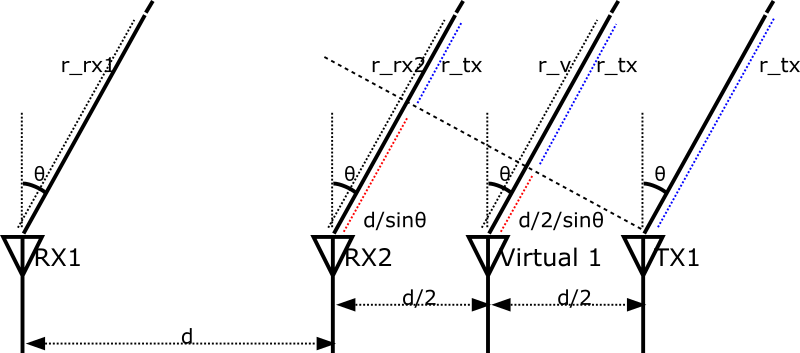
Figure 6-1 illustrates the time-of-flight difference between the different antennas.

Figure 6-1 MIMO Illustration of phase increases for each receive antenna.

At a high level, the angle of arrival is derived from the difference of time of flight measured at each receive antenna.

At the mathematical level, from each antenna Equation 6 defines a steering vector as:

Equation 6.

a (θ) = [e^{j \times 2 π \times d \times \frac{s i n (θ)}{λ}} e^{j \times 2 π \times d \times 2 \times \frac{s i n (θ)}{λ}} e^{j \times 2 π \times d \times 3 \times \frac{s i n (θ)}{λ}} \dots e^{j \times 2 π \times d \times N \times \frac{s i n (θ)}{λ}}]

The steering vector is used to combine the signal from each target at each antenna. In Equation 7, which expresses the sum of all signals coming from each target through all antennas, x_i is the signal received by the i’th antenna:

Equation 7.

y (t) = a^{H} x (t) = \sum_{1}^{N} a_{i} \times x_{i} (t)

Equation 8 calculates the average power as:

Equation 8.

P (a) = \frac{1}{L} \times \sum_{1}^{N} | y (t) |^{2} = a^{H} E {x (t) \times x^{H} (t)} a = a^{H} R a

Conventional receive beamforming, also known as the Bartlett beamforming method, is the oldest direction-of-arrival estimation algorithm based on narrowband arrays. This algorithm maximizes the output power of the beamformer relative to a certain direction, expressing the maximization relationship in Equation 9 as:

Equation 9.

θ_{B a r l e t t} = a r g m a x_{a} [P (a)]

To compute P(a(theta)) for each theta, Equation 10 approximates R as:

Equation 10.

R_{z z} \approx \sum_{k = 0}^{n} X (t) \times X^{H} (t)

where X is the matrix of signals (Equation 11):

Equation 11.

X (t) = (\begin{matrix} \begin{matrix} x_{1} (t_{1}) x_{1} (t_{2}) \dots x_{1} (t_{n}) \\ x_{1} (t_{1}) x_{1} (t_{2}) \dots x_{1} (t_{n}) \end{matrix} \\ ⋮ ⋮ ⋱ ⋮ \\ x_{M} (t_{1}) x_{M} (t_{2}) \dots x_{M} (t_{n}) \end{matrix})

From these equations, you can see how a MIMO radar enables location derivation in three dimensions.