SBOA537 March 2022 TMP61 , TMP61-Q1 , TMP63 , TMP63-Q1 , TMP64 , TMP64-Q1
4 Creating a Polynomial for the Collected Data
Polynomial curve fitting is the process of constructing a curve or mathematical function that has the best fit to a series of data points. In mathematics, a polynomial is an expression consisting of indeterminates and coefficients, that involves only the operations of addition, subtraction, multiplication, and non-negative integer exponentiation of variables. In theory, the polynomial coefficients are always positive and the function has operations of addition, subtraction, and multiplication. The goal in programming is to fix the code and only have to change out the coefficients. A polynomial equation is modified in code to only use addition and multiplication so that the formula remains constant. So positive and negative coefficients are used to perform the addition and subtraction needed. For the TMP6 parts, a 4th-order polynomial is used to get the best curve fit for the near linear curve of the PTC thermistor.
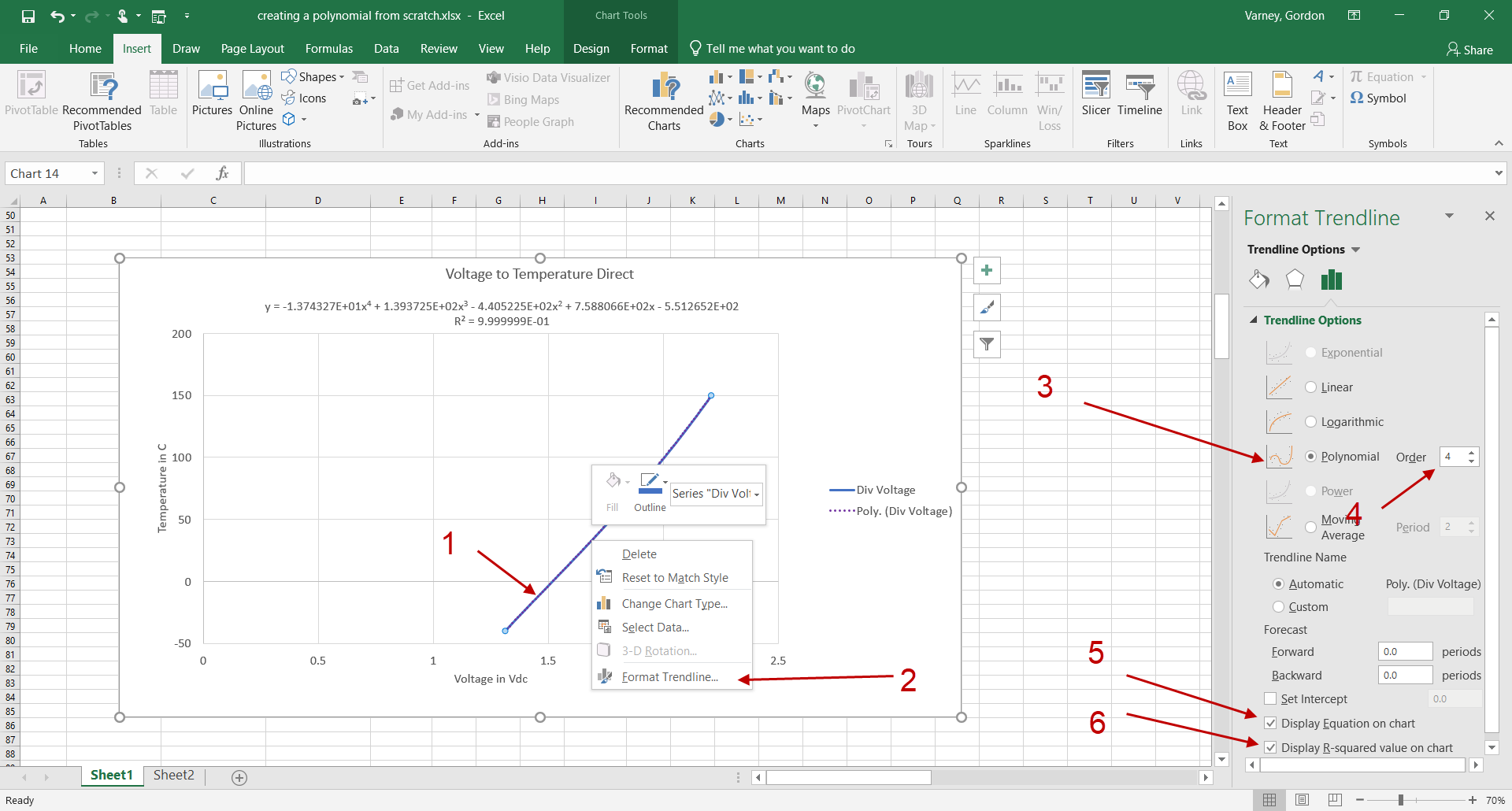
Use the following steps to create the polynomial from the Microsoft Excel scatter plot previously created. Follow the flow in Figure 4-1 for each step of the process.
- Right click the plot line
- Select Add Trendline, then the trendline must be formatted
- Select the Polynomial trendline option
- Change the Order to "4", for 4th-order
- Check the box for Display Equation on chart
- Check the box for Display R-squared value on chart
 Figure 4-1 Polynomial Flow
Use 6 digits of precision in the coefficients to maintain the accuracy of the calculations as much as possible. Figure 4-2 shows how to change the format of the label to get the required digits for the coefficients.
- Right click the label for the polynomial and select Format Trendline Label
- Change the category to scientific
- Change the number of decimal places to "6"
 Figure 4-2 Format the Trendline
Label
Figure 4-2 Format the Trendline
LabelNow you can copy the formula and the coefficients from the trendline label and paste it as text in a spreadsheet.
where
- V = ADC Voltage
- A4 = –1.374327E+01
- A3 = 1.393725E+02
- A2 = –4.405225E+02
- A1 = 7.588066E+02
- A0 = –5.512652E+02
Remember that if the formula requires the subtraction of a number, keep the (–) minus symbol with the coefficient. Now the polynomial formula can be created in code with only addition as in the main polynomial in Equation 1. Adding a negative number is the same as subtracting.
Now replace the X4 through X values with the measured ADC voltage in the polynomial formula. Use the coefficients you created in the new formula.