SLVUC15 March 2021 TPS7H4001-SP
3.2 Monte Carlo
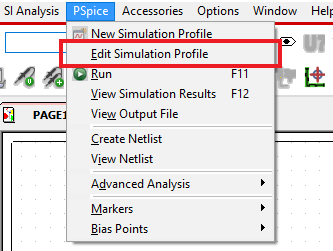
- Edit the frequency response simulation profile created in Section 3.1 by clicking
on PSpice → Edit Simulation Profile.
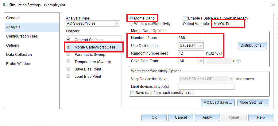
- In addition to the parameters that were previously set in the
General Settings section, the following parameters will also need to
be set in order to run Monte Carlo simulation:
- Monte Carlo/Worst Case
- Select the "Monte Carlo" simulation option
- Define the signal that will be analyzed as the Output Variable (VOUT is used in the example below)
- Set the number of simulations to run
- Select "Gaussian" for the distribution
- Enter a value for the random number seed between 1 and 32,767 if a specific set of random simulations is desired (otherwise this field can be left blank)
- Monte Carlo/Worst Case
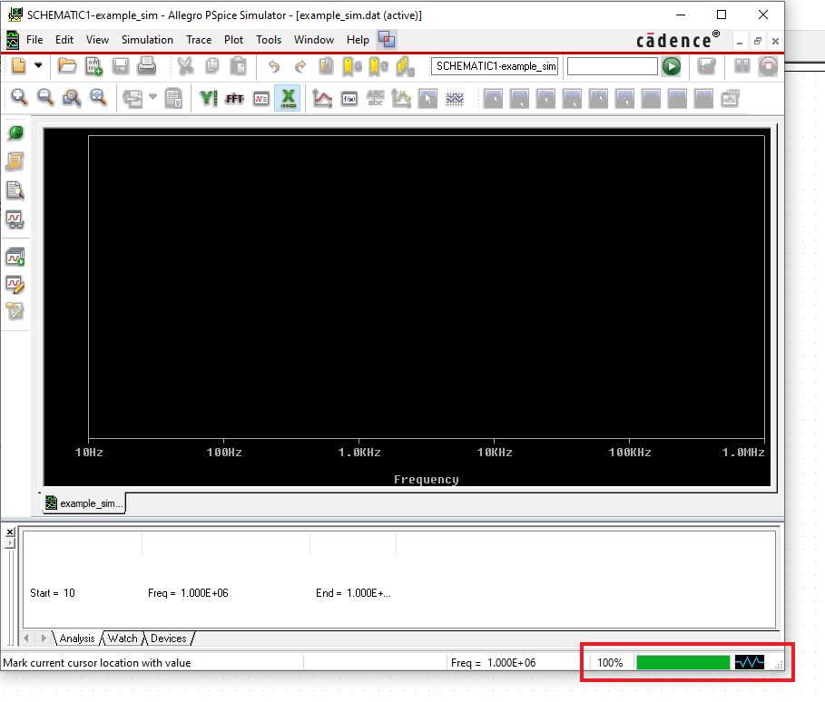
- Run the simulation by pressing F11 or
PSpice → Run. The simulation window will open and simulation progress
will be shown in the bottom-right corner.
- After the simulations are complete, a window will appear that lists them all. Press OK. The frequency response results can be viewed as a Bode plot by following the directions in Section 3.1 starting from step 6.
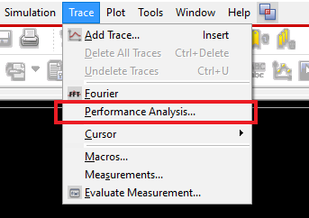
- In order to view the results as a
histogram, select Trace → Performance Analysis. A pop-up will appear.
Click OK.
- Right click on the plot area and click Add Trace.
- Once again, the desired signal
and display method can be chosen. For example, phase margin can be displayed by
entering the following expression into the Trace Expression field:
PhaseMargin(DB(V(VOUT)),P(V(VOUT)))-180
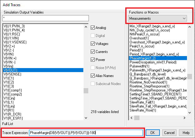
- Click OK and the histogram will be displayed along with statistical information that describes the distribution of the simulation results, such as min, max, standard deviation, and mean.
 Figure 3-2 Monte Carlo Histogram of Phase
Margin
Figure 3-2 Monte Carlo Histogram of Phase
Margin